LAB SESSION 10
ANALYZING MEAN
AND VARIANCE (SIGMA UNKNOWN)
INTRODUCTION: The t-statistic is used when making inferences concerning the population mean when sigma is an unknown quantity. We will introduce the t-test and compare the z and t distributions.
THE CONFIDENCE INTERVAL
To generate a confidence interval using the t-statistic we use Inference About a Mean command, specifying the level of confidence and the column of data for which the estimation is being made.
Consider the data presented in exercise 9.35 of your text. Enter the data into Column A. To complete a 90% confidence interval estimate for the mean pulse rate for 13 adult women, use the following commands:
Enter the data into Column A
Choose: Tools > Data Analysis Plus
> t-Estimate:Mean > OK
Enter: Input Range: A1:A20 > OK
Enter: Alpha: .05
The results in the following output which appears in a new worksheet.
|
||||||||||||||||||||||||||||
THE TTEST
Using text exercise 9.34 as the basis of our discussion, enter the data values into column A. Suppose we have been asked to determine whether this accelerator has decreased the drying time by significantly more then 4% at the 0.01 level. The hypotheses to be tested are:
H0: µ = 4.0
Ha: µ > 4.0
To perform the test, use the following commands:
Enter the data into Column A
Choose: Tools > Data Analysis Plus
> t-Test Mean > OK
Enter: Input Range: A1:A20 > OK
Hypothesized mean: m
Alpha: a > OK
The output appears on a new worksheet as follows:
|
t-Test: Mean |
|
|
|
|
|
|
|
|
|
|
|
|
Column 1 |
|
Mean |
|
|
4.5625 |
|
Standard
Deviation |
|
1.3405 |
|
|
Hypothesized
Mean |
|
4 |
|
|
df |
|
|
7 |
|
t Stat |
|
|
1.1869 |
|
P(T<=t)
one-tail |
|
0.137 |
|
|
t Critical
one-tail |
|
2.9979 |
|
|
P(T<=t)
two-tail |
|
0.274 |
|
|
t Critical
two-tail |
|
3.4995 |
|
Is there sufficient evidence to show that this accelerator has decreased the drying time significantly more than 4% at the .01 level?
As another example consider the point spread between opposing teams in the 1996 bowl games : 5 20 19 33 6 10 7 18 29 41 6 32 9 36.
Enter the data into Column A.
Test the hypothesis, "The average spread between the scores of the winning and the losing teams in a college bowl game is less than 20." Assume sigma is unknown.
Use the same commands as above to get the following output:
|
t-Test: Mean |
|
|
|
|
|
|
|
|
|
|
|
|
Column 1 |
|
Mean |
|
|
19.3571 |
|
Standard
Deviation |
|
12.7013 |
|
|
Hypothesized
Mean |
|
20 |
|
|
df |
|
|
13 |
|
t Stat |
|
|
-0.1894 |
|
P(T<=t)
one-tail |
|
0.4264 |
|
|
t Critical
one-tail |
|
2.6503 |
|
|
P(T<=t)
two-tail |
|
0.8528 |
|
|
t Critical
two-tail |
|
3.0123 |
|
|
|
|
|
|
Questions:
1 What are the formal null and alternative hypotheses?
2. What is the value of the test statistic, and what is your decision if a = .10? Is the final point spread of a bowl game less than 20?
3. What does the size of the p-value tell us?
ASSIGNMENT: Do Exercises 9.46, 9.49 in your text
COMPARISON OF THE Z AND T DISTRIBUTION
Why do you use two different distributions depending on the availability of the standard deviation, s ? What basic assumptions are necessary to use the t-statistic? Is the basic assumption that the parent population is normally distributed a necessary one? Why? If the parent population is not known to be normally distributed, when can we use the t-statistic? In this exercise you will generate both types of statistics from the same 100 samples and be able to compare the two empirical distributions.
In a new workbook, generate 100 samples of size 5 from a normal distribution with mu=15 and sigma=10, and store the mean and standard deviation of each of the 100 samples.
Choose:
Tools > Data Analysis > Random Number generation > OK
Enter: Number of Variables: 5
Number of Random Numbers: 100
Distribution: Normal
Mean: 15
Standard Deviation: 10
Select:
Output Options: Output Range > A1 > OK
This will make 5 columns of 100 random numbers each.
Calculate the Mean and Standard Deviation of each row and place them in columns F and G. (Do this for row 1, and click and drag to fill the remainder.)
Calculate both z and t statistics of each row and place them in H and I.
Recall:  and
and 
Replicate these for all 100 rows by highlighting and dragging the lower right corner.
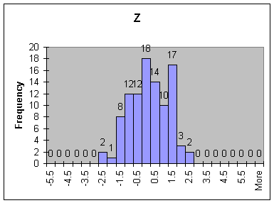
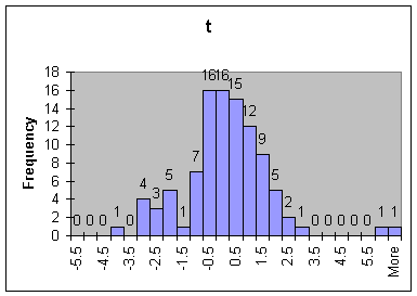
For each of the two statistics, z and t, count the number of times their value is more than 2 units away from the origin.
Compare the two distributions graphically by using histograms (recall the method from Lab 2)


QUESTIONS:
1. How many of the calculated z-statistics were more than two units away from the origin? How many of the t-statistics?
2. What did the distributions for the two statistics look like? Compare their centers, spread, and overall shape.
3. Would you describe the t-distribution as bell-shaped? If so, would you say it is approximately normal?
4. If you were to increase n, would you expect the difference between the two distributions to increase or decrease?
ASSIGNMENT: Do Exercise 9.50 in your text.